Table of Contents

Intro

Recently I began studying FMCW Radar in my spare time with the goal of simulating it. Compared to pulsed radar, FMCW radar is more common, because it can be built with smaller & less expensive components.

I want to write down what I learned and key take aways are.

link

Concept & Key Ideas

FMCW (frequency modulated continuous wave) radar is unlike pulsed radar (effectively listening for an echo) using a continuous wave. It deteremines the distance to a target by measuring the beat signal that one gets from mixing the transmit and return signal. The velocity can be measured either via the doppler shift or by phase. In this post I will focus on doppler.

When multiplying two signals of similar frequencies you get a signal made of two very different frequencies.

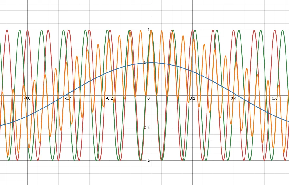
The plot shows two signals red & green with both similar frequency ($f_1$ and $f_2$). Multiplying both together gives you the orange signal. The low frequency (called beat frequency) component can be extracted with a low pass filter. With the beat frequency $f_b$ one can derive distance and velocity.

Also described mathematically

Where $\alpha = 2\pi f_1 t$ and $\beta = 2\pi f_2 t$ and thus $f_b = f_1-f_2$.

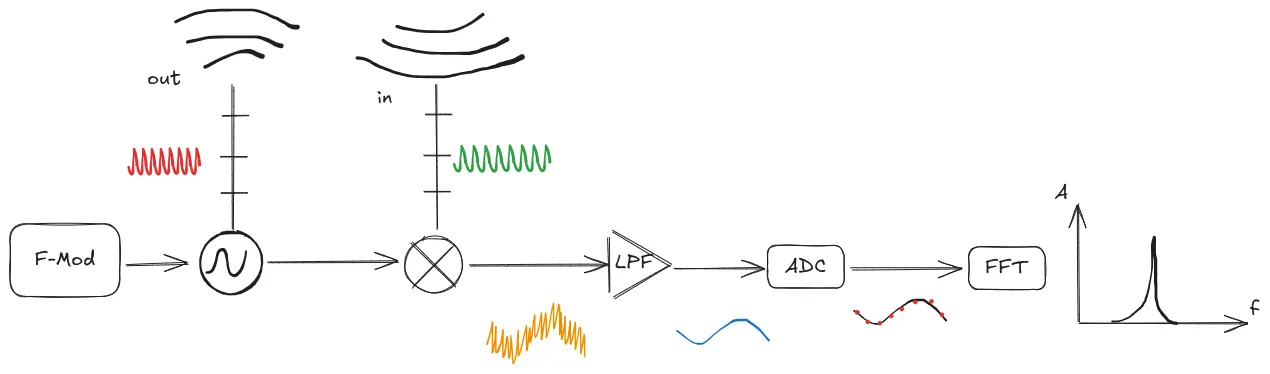
Applied to FMCW: the antenna sends out for example the red signal and the receiver picks up the green signal. A mixer mixes the two frequencies and we get orange. It has too high of a frequency for us to measure the signal. Therefore we use a low pass filter to get just the beat frequency signal. That we then pass into an ADC (analog digital converter) and using an FFT (fast fourier transform) determine the beat frequency.

Why is the green signal different?

Two reasons:

1. The first is doppler frequency shift due to velocity of the target $f_d = \frac{c-v}{c+v}f_0$. Not gonna explain here; covered enough elsewhere.
2. You may have noticed F-Mod (Frequency modulator) in the image above. It creates a chirp (signal with increasing frequency). As the signal travels to the target and gets reflected back, the carrier frequency with which the reflected singal will be mixed with increases, which like seen above produces a beat frequency.

How does one measure the target range $r$ from beat frequency?

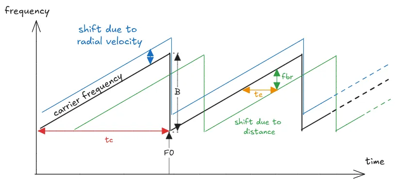
Let’s say the chirp sweeps the bandwidth $B$ within chirp time $\tau_c$. The signal is sent out at the speed of light $c$ and reflected off the target. After some time $\tau_e = \frac{2r}{c}$ it will echo back at the frequency it has been sent out $f_{c1}$; however by now the carrier frequency $f_{c2}$ has changed, because the frequency modulator increases the carrier frequency (chirp). We mix, lowpass, sample, fft the signal and extract the beat frequency due to range $f_{br} = f_{c1} - f_{c2}$.

The plot above shows the red carrier frequency and the The plot above shows that $f_{br}$ and $\tau_e$ form a triangle. From the graphic above we know that

$\frac{f_{br}}{\tau_e} = \frac{B}{\tau_c} \implies \tau_e = \frac{f_{br}}{B}\tau_c$

We know how long we expect the echo to take $\tau_e = \frac{2r}{c}$ and how long it actually took $\tau_e = \frac{f_{br}}{B}\tau_c$. That’s all we need to determine the range

$r = \frac{f_{br}}{B}\frac{c}{2}\tau_c$

🤔 But isn’t the signal also changed by the doppler frequency? How do we know its range and not doppler?

$f_b = f_{bd} + f_{br}$

Yes! Which is why we use not only one chirp time but multiple.

$f_{b1}$ we measure for chirp $\tau_{c1}$ and $f_{b2}$ for chirp $\tau_{c2}$. This will give us two equations.

$f_{b1} = f_{bd1} + f_{br1}$

$f_{b2} = f_{bd2} + f_{br2}$

Let’s quickly talk doppler to identify the doppler frequency shift $f_{bd}$. The signal is sent out at $f_{c1}$. It gets doppler shifted to $f_d = \frac{c-v}{c+v}f_{c1}$ and then arrives back while the transmitter is already at $f_{c2}$ due to chirp. We measure the frequency difference between carrier and received signal the same way we did with range, therefore the doppler shift is

In real world applications $f_{c2} \ll f_{br}$ and therefore it can be simplified $f_{bd} = 1 - \frac{c-v}{c+v}$. Therefore $f_{bd1} = f_{bd2}$.

$f_{b1} = f_{bd} + f_{br1}$

$f_{b2} = f_{bd} + f_{br2}$

Plugging into the equations and shuffling around

$f_{b2} - f_{b1} = f_{br2} - f_{br1} = \frac{2rB}{c\tau_{c2}} - \frac{2rB}{c\tau_{c1}} = r\frac{2B}{c}\left(\frac{1}{\tau_{c2}} - \frac{1}{\tau_{c1}}\right)$

$r = \frac{c}{2B}\frac{f_{b2} - f_{b1}}{\frac{1}{\tau_{c2}} - \frac{1}{\tau_{c1}}}$

From this we can find a range and velocity for two beat frequencies. One could also use triangular frequency modulation.

That’s the core principle of FMCW radar.

Note: In reality this approach is not very practical, because you would need a set of chirp pairs for each each object reflecting signals into the radar receiver. Nevertheless understanding this approach helped me with the more advanced I will demo some other time.

Demonstration

You can interact with a live FMCW radar simulation below. Where the lines in the top plot cross is where the radar would measure a target.

Major caveats:

• The intensity of the echo signal decays with $\frac{1}{R⁴}$. Therefore targets would barely be visible.
• No Noise

Regardless, the principle is visible. Some components that are not shown in other descriptions.

Some things to try:

• as you move the objects see how the peak in the fft moves. We can determine the location from that peak.
• change the second chirp duration. You will get more different peaks
• as you increase the bandwidth the beat frequencies grow too
• change the sampling duration. Note how the peaks become slimmer
• move an object until it’s peaks go beyond the fft (it looks as if they get reflected). This is how aliasing looks like in fft
• as you reduce sampling frequency, you get less maximum resolution

And lastly changing velocity doesn’t do much with most parameter combinations. A way to alleviate this problem is with another approach, I might describe in another article.

Conclusion

I really enjoyed this deep-dive into a topic. Doesn’t feel stressful when there is no exams. I hadn’t felt so many great “Aha!” feelings in some time. Considering that Signal Theory is now almost 5 years ago I picked it back up quite quickly (guess the ability to learn fast is really one of my strengths).

In a future article I will do this with another approach, that is more common. I hope to get something I can build something from.